Is’ useful at this point, a recall on processing techniques with the tools at the sub-diameter, in particular on how it is possible increase the curvature of one or more zones.
Then resume the concept according to which through sub-diameter strokes , External areas increase their curvature while those inside the decrease, which is to say that during the past generate a “furrow” on surface, where the central sector of the machined area is deeper than the rest of the surface not machined.
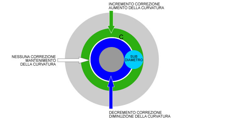
Fig. 1 – Action on the diameter of the sub-surface curvature
In theory ( but not in practice ) the only application of this technique is sufficient to achieve the desired result. we see how:
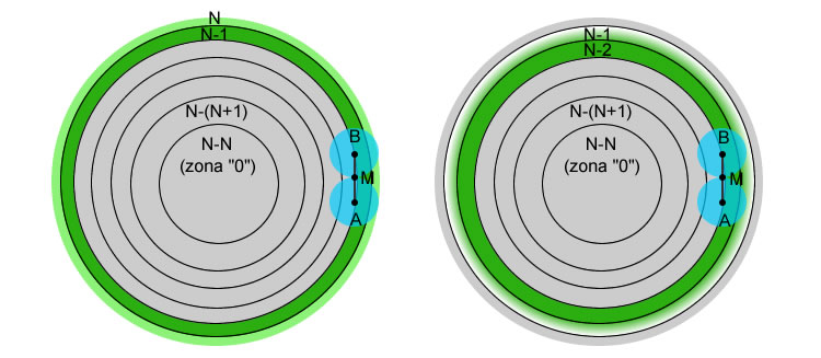
Fig. 2 – Sequence of the curvature increases in adjacent areas.
We assume N as the total number of areas in which virtually divide our mirror . So we will have our succession of zones ( circular sectors of default width ) starting from the edge toward the center mirror: N, N-1, N-2, ….. , N-N.
Our starting hypothesis tells us that sphere and parabola are coincident in the edge, but given that in the tests we will never have a way to measure the curvature in the edge, nothing prevents us from “to shift” This point of tangency ( remember that can be chosen in an arbitrary manner in any point of the spherical section starting ) at the center of the most peripheral area ( N ) , just at the point where the measurement is carried out.
We will have so that the center of the last zone is by definition “correct”, being tangent to both the ball to the parabolic profile of the project and therefore must not be worked, then we begin to excavate the center of the next area N-1 until also not be tangent to the parabolic profile wanted.
To do this we must make the area N-1 and its deeper center of one of the area N compared to the starting sphere, in other words we need to increase the curvature of the initial ball moving from N-1 until N.
then applying the aforementioned diameter of the sub-technique, We prepare a tool whose radius is slightly greater than the distance between the centers of two successive zones , We will position the tool center on the inner edge of the area N-1 and will perform small rides to and fro with circular pattern all around the area. The result will be that we will have increased the curvature exactly between the area N-1 ed N. We will make the measure of this increase with a suitable test, limiting ourselves to only measure the “draft” of these two zones, and we repeat sessions with the sub-diameter until the draft measurement will not be coincident with that of the simulation ( calculated mathematically or via software ) of our final parable .
At this point we have two correct areas than the end parable. then we will pass to the next zone N-2 and repeat the same procedure “excavation” and connection between the N-1 and N-2 up to bring this also draw to the correct value.
We will apply the procedure in succession until the last area N-N ( the center of the mirror or “zone 0” ) to ensure that the last zone “helpful” , the N-(N+1) , which is the first central area , Full configuration and connection of the parable.
WITHIN THE “TRUMPET OF TOLERANCE”
the generation of the parabola as increasing deepening of consecutive zones, It can also be seen as a succession of flow areas “tolerance” in Millies-Lacroix graph. To do this we must resort to a small “makeup” that will help us in the immediate view of what you're going to do.
Our starting sphere with identical radii of curvature of the zones ( draw = 0 ) inserted into ML graph of a hypothetical mirror 300 mm F4 parabolic, He would have a representation similar to this:
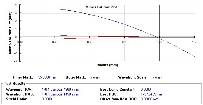
Fig. 3 – Millies-Lacroix Chart for a spherical surface ( the scale is altered for better viewing )
Let us now apply our first hypothesis, namely, that of tangency between the edge of the sphere and parabola,( instead of the radius 115 mm as shown in Figure) , which is equivalent to translate the upward curve up to the dropping of the radius curvature center 150 mm at the center of the tolerance trumpet:
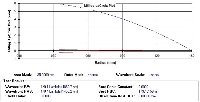
Fig. 4 – Millies-Lacroix Chart for a spherical surface tangent to the edge with the ideal paraboloid ( the scale is altered for better viewing )
the translation ( the “makeup” ) we just did on Ml Chart match what we chose to do in Section B of first part of:
B - "We shorten" the central reflections: It is tantamount to saying that, starting from the edge and we move gradually towards the center will increase the curvature of the mirror in such a way that the reflections of the central zones converge closer, just enough to make them coincide with those devices.
Looking at the chart set up this way, is quite intuitive that, to bring the ball to the parable, the entire curve will go into tolerance, We must therefore deepen the surface (“tear down” the curve ) increasingly starting from the edge toward the center
Suppose we have calculated the exact values of the centers of curvature of our ideal parable and work the mirror according to the procedure, bringing first the exact radius of curvature of the area N-1 ( in this example N=5 ) and then all the other. Here's what we should expect in the ML graph calculated using the test in Foucault, ie the sequence of the corrections area after area :
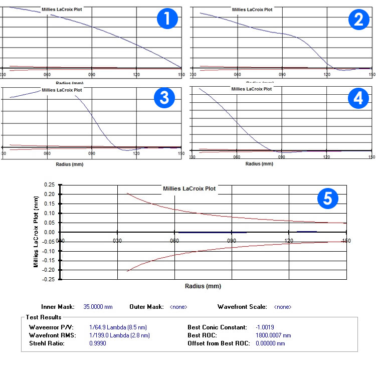
Fig. 5 – Succession of zonal insights.
FROM THEORY TO PRACTICE
As mentioned, in the practical realization things are not immediate, They intervene in fact different elements that advise against such a direct approach, to be found in advance of the solutions to these problems:
- for short focal lengths, the number of areas to be examined must be reasonably high, the greater the number of zones is less than the extension of the tool that allows to work only two adjacent zones without interfering with the other, deducible with increments of processing times.
- Increasing the curvature of the outer area decreases accordingly that of the inner area which will subsequently be thorough both value with respect to the sphere of the additional value of decrease of the curvature newly generated.
- the lower the tool extension, the greater the likelihood of generating local surface errors of difficult correction, the “little ones” sub-diameter should be used sparingly , for small corrections and a good experience to use in less configurations “extreme”.
- It is difficult to arrive at the exact measure of the draw of two zones acting in one direction only, namely only the increase of the curvature. Is’ probably closer to the ideal figure will exceed ( although very little ) in the processing and it is necessary to “come back” ie acting in the opposite direction to decrease the curvature, with direct and unavoidable consequence of modification of form also on the adjacent areas.
- This procedure does not allow a comprehensive inspection of the surface during the construction of the figure, especially with the complementary tests as the Ronchi, It is based on “confidence” that we are working well, but confirmation will come only after completing the entire parable.
This last point can best be highlighted if we simulate the graph of Test Ronchi corresponding to the processing area after area phases:
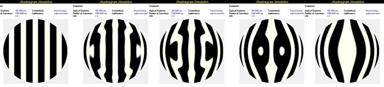
Fig. 6 – Simulation of the Ronchi Test for the deepening succession zonal.
As you can see in Figure 6 , this methodology while maintaining good initial premises, It does not allow to immediately assess how much the machining on both “right stada”, only after having brought all the custom zones, we will evaluate the surface correction in its entirety.
It is therefore necessary to optimize this strategy throughout the construction work of the figure, to make possible the machining quality control during each phase, eliminating or at least minimizing the possibility of local or general errors and still allowing to identify them with certainty and to intervene “insecurity” if it presentassero.
Is’ what we will find out in the third part.