
As described in the previous article entitled "Preparatory phase to Foucault's test", We have prepared the room, with mirror aligned and testers on their tables and stands, left to acclimatize the mirror to reach the safe thermal equilibrium with the ambient temperature, and now we are ready to begin the first test session.
We take our paper notebook in which we had recorded the following (see image) table of 4 rows and 5 columns copied from the mask Couder
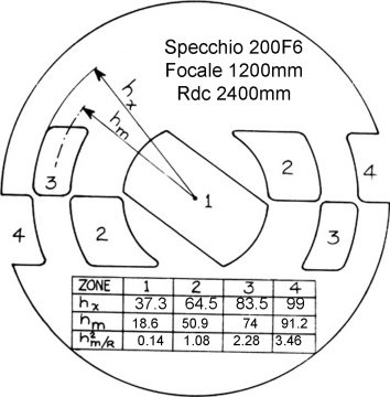
Where the values of hx and of hm of each zone (see rays which it comes in the image of the mask here above) were given as construction data in the same mask, while in the calculation of hm 2 /R appear R, that is the radius of curvature of 2400 mm, corresponding to the focal length estimated of 1200 mm of our mirror, that may be corrected exactly at the millimeter when we exactly measure.
We mark the notebook page that relates to the test No. 1, as Page # 1, and we continue the vertical lines of the fincature table continuing their lines up at the bottom of the page, as in the following image. (Ma, as we'll see, to facilitate the design of the final graph, is better if 4 columns that relate to 4 zones, It is immediately set with equal width of 10 paper squares ).

We turn on the source and align KNIFE AND SLIT
Attention that from this moment on it is important to ensure that the position of the tester don't move with respect to the mirror in question, always keep its alignment, as it is perfected by bringing the blade of the knife to “to cut” the light rays coming from the center of the radius of curvature of the central area of the mirror, which is the starting point of the Foucault test.
Then We put ourselves in observation position behind the tester.
Since we had positioned the tester aligned to the mirror and already very much “close” the radius of curvature 2400 mm belonging to its focal length, looking at the mirror from behind the tester blade, we see it fully illuminated; that is, we will see that the light of the slit, put at that distance “nearby” the radius of curvature, It is diffused over the entire surface (which is not the case otherwise).
NOTE: To see how you perform in practice the alignment between mirror and tester, the vision we recommend 4 minutes (manually setting it from the point “1 hour 04 minutes”, to the point “1 hour 08 minutes”), of the following movie .
-Considering also that to trace the image of the slit, in return from the mirror reflection, It is more convenient to remove that slit in front of the LED, so that we can more easily search for the more visible “cue ball” bright of the led reflection, no longer hidden by the slit;
-And also, instead of using a small translucent screen as seen in the movie, it is more convenient to use a simple sheet of cardboard to traverse to track the reflection, and complete the alignment of the tester, carrying that bright led disk, exactly on the tester blade. END OF NOTE.
If now we turn our head back a foot, and we put a lens (no matter focal lenght) in the position where before we had the eye, We will see the image of the slit appearing on the glass of the lens (see pictures).
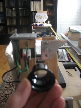

The image of the clear slit, that have on it right, the one of the grey blade knife edge that must be adjusted exactly parallel to it
We then move the blade forward (that is to the left) so as to make it appear to the right of the slit and carry it forward until we reach the edge of it.
Now we set the orientation of the blade knife edge so that the blade and slit are parallel.
Advancing the blade check that the slit light will turn off extinguishing itself from top to bottom at the same time.
Note that when the blade advances are so tiny to do (something that also happens in normal surveys with tester) it is much more comfortable to use its adjustment screw, but press with two fingers on the base of the blade holder, that, with its little elastic bending, will absolve the desired task.
LIGHTING ENVIRONMENT TEST
We prepare the most convenient ambient lighting to allow the minimum eye fatigue and the maximum contrast sensitivity, creating semi-darkness so similar to when you watch TV. A head lamp, red light (or in any case not so much powerful light to annoy the eye) Let us read well on the micrometer forwards and backwards movement of the tester trolley, reading values to register on notebook.
MEASUREMENT BENDING RADIUS AND FOCAL MIRROR IN REVIEW
If after checking the blade - slit parallelism, Insert completely that last in the light cone, we will see its image projected on the side of the blade opposite the mirror, we'll be able to maneuver the cart forward or backward tester in order to improve the focus of that image.
Once you have reached the point of best focus, you need to get someone to help you measure with precision to the millimeter without moving any component of the installed setup, the distance between the center mirror and blade, and also the distance between the slit and mirror center. The arithmetic average of the sum of the two values is the radius of curvature of the mirror, that is twice the size of its focal distance.
But there is another more accurate way to find the focal length of the mirror, and that is to seek the “flat grey colour” that is the center of curvature of its zone 1, that appears in the center window of the Couder mask, starting the first round of surveys of the reading zones. that is in fact The first session of the Foucault test.
The zone 1 is that of the central mirror,and it is the most critical and challenging to measure, as mentioned earlier in the article entitled "FOUCAULT TEST WHAT IT IS AND HOW IT WORKS"
Is’ criticism because it is the place of departure which will refer all our measures from zone to zone, and is therefore the most important because wrongly assumed that,, There we take you behind the error on all other zones.
Is’ challenging because is the largest but is also the least deformed, and thus requires the most moving lengthwise tester cart compared to other zones that will be examined, but the worst is that in this great movement, always seems that the shadow visible changes little or nothing, due to the little local deformation.
This therefore makes it really difficult to identify, in those shades of gray seemingly always equals, which is the famous “flat grey colour” that matches exactly the focus of the zone.
Every operator who runs into that mistake, Learn at his own expense, and creates its own thumb rules to find out with certainty the exact focus.
My rule is as follows:
- Move the tester carriage ONLY longitudinally towards the mirror (operating with its longitudinal adjustment screw on the optical axis of the mirror) in a frankly intrafocal area (that is, closer to the mirror than the expected curvature cetro), and introduce the blade (operand with its orthogonal adjustment screw) in such a way that it reaches the center of the mirror, and annotate the longitudinal draw of that starting point, Readed on the measuring micrometer carriage back and forth movement of the Foucault tester. With a tester “standard”, (namely, that introduces the blade from right to left, view by the operator behind the tester), the shadow intrafocus view on the mirror it will reach its center coming from the right: Suppose you read at that point the value 55.96mm.
- Leave the blade in that position and move backwards only with the longitudinal trolley moving away from the mirror until the shadow of the blade becomes visible. the same position mirror symmetrical with respect to the first (that is, as you move away from the mirror, the shadow of the blade will be seen arriving at the same point, but from left to right), and note the draw of that point of arrival extrafocale: Since our tester was built in the "standard", that in addition to providing for the introduction of the blade from right to left, provides the increase of the micrometer readings with the departure of the trolley from the mirror, Suppose we read at that point 62.20mm.
To difference of the two values (62.20-55.96=6.24mm) there is the draft distance from the initial intrafocal position to the homologous extrafocal final position. Dividing by two we find (6.24/2=)3.12mm which, added to the distance between the starting position 55.96 It provides (55.96+3.12=) 59.08, which it is the extent to which move the carriage of the tester.
If everything went smoothly, that position remote cart 59.08 mm is the location of the center of curvature of the zone 1, and we can verify it while watching the shadow will extract and reinstate the blade finding the presence of “flat grey colour” date from closing gray shadow concentrically and evenly, backgrounds without showing it neither from the right nor from the left.
Aided by someone we measure now the distance center mirror – blade , and We Add at the distance center Mirror - slit , and divide by two, finding 2400 mm radius R of curvature, and with this value R we correct the values of hm 2 /R in the boxes on our notebook.
Having found the focal length of the mirror (corresponding to R/2) do not forget to write down on our notebook, the draw of the detected value for the area n ° 1 of our 200F6 , we read to be 30.89mm. Do not move the tester because we will continue from that location for the Centre of curvature in the other three zones more an more peripheral.
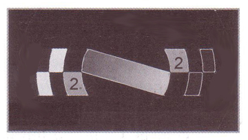
TEST IN Foucault: Examples of shadows that arise operator.
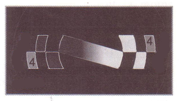
The observation of spot colors in many zones, orientativamente would occur as in the following 4 inìmages, in which the number inside the window, It indicates its spot.
Note 1:
For example: In the image of the zone 1 (virtually imaginable area as it also consists of two windows, one on the right and one on the left of the mirror center), you notice that the two parts right and left are in uniform “flat grey colour”, and the shadows are all in the areas to his right of the. That is, in them we find ourselves in intrafocal, or BEFORE the fire corresponding to those peripheral areas (which in fact are unbalanced in gray a little different from the flat color, for the zone 2), but we're also a lot more intrafocus in the Windows of zones 3 e 4, which therefore at the moment are still in very dark gray on the right and white on the left.
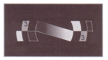
Note 2:
We look at the central window (zone 1) in the pictures after the first, and we see increasingly darken, from left to right, as we increasingly control the peripheral zones. Which clearly indicates that, at that time, the zone 1 is already in clear position extrafococus relative to the current point of the measurements. And they will be in uniform spot color, gradually the pairs of windows of the other areas.

WE THEN ACTUALLY EXECUTES THE TESTING
on the mirror 200F6, with the search for FLAT GREY COLOURS of all four zones, starting from the zone 1 in departure from the mirror, up to the zone 4, with the notation of their drawdowns on the notebook.
- Once detected the zones 1,2,3,4, We distance ourselves a little empty, for beginning to reverse then the detection direction, and go back to the mirror, for a second series of detections, of the zones 4,3,2,1.
- Returned back to the zone 1, We are still a little empty for reversing again the sense of measuring to a third data series, on the zoners 1,2,3,4 and going on a little farther.
- And finally, we reverse the last time to record the last set of the zone data 4,3,2,1.
Eventually we will have the following four sets of values to be averaged:
| Zone | Z1 | Z2 | Z3 | Z4 |
| Round 1 | 30.89 | 31.39 | 31.74 | 31.9 |
| Return 1 | 31 | 31.43 | 31.86 | 32 |
| Round 2 | 31.2 | 31.52 | 31.82 | 32.11 |
| Return 2 | 30.91 | 31.68 | 31.8 | 31.99 |
| Media | 31 | 31.5 | 31.8 | 32 |
Values that we will use for the evaluation of the surface, we had already registered on our notebook during and surveys, as in the following image, in the box in red.

The average of the four test series, you why "fix" the errors committed in the evaluation of a non-expert, greatly increasing the reliability of the calculation that will run with them. However, the experienced operator could easily non take four values but limiting at two, or reduce it to a single round-trip.
Returning to our numbers:
We have at our disposal before, the values of hm 2 /R representing the longitudinal aberration of the perfect reference parabola with focal 1200 and Radius 2400mm, which it would pass with those values exactly in the centers of the windows of our Couder mask: Aberration values that were as follows.
For the perfect reference parable:
| zone | 1 | 2 | 3 | 4 |
| Aberration | 0.14 | 1.08 | 2.28 | 3.46 |
(NOTE: It pays to remember that they are called optical aberrations, the quantities of the”deformations” of the original sphere which achieve the desired parabola. Normally, in common parlance, the term “aberration” it is derogatory. But in opticals they are the positive qualities that should be imprinted in the original sphere glass, to get the desired parabola).
And now we just found our average values of “draft” or named aberrations “still rough”, 31 ; 31.5 ; 31.8 ; 32 , because they differ from the reference values0.14 ; 1.08 ; 2.28 ; 3.46 , because on ours, is added a unknown constant , due to the scale reading on our micrometer measurement, which it could in no way be synchronized with the calculation values of the theoretical aberration.
So we find that constant to be able to subtract with our measurements to "bring closer" as possible to the reference values in order to make the comparison with them easier and obvious.
PAUSE FOR AN INTERESTING REASONING:
Since in general it is convenient (for the less quantity of glass to scratch), parabolizzare from 70% the diameter, and since the radius of the mirror we call technically hm, in our case we infer that the radius belonging to 140mm diameter falls in the area 3 of our mask, who have hm = 74.
Imposing that point lyke of contact point, Basically we assume that the zone 3 is perfect (I.E. having zero aberration difference, i.e. it coincides with the perfect parable of reference). And this will allow us to see how and what, the other zones are moving away (that are the errors) from the values of the perfect parable of reference.
(Note that we may very well and lawfully do the same thing as the contact zone and reference "zero", any of the other zones of the mirror. But this in general is never convenient for too much work resulting ... unless special cases in which we can recover a mistake clumsily committed, otherwise difficult to eliminate).
END OF REASONING
THEN APPLY OUR INTENTIONS
To "move" in mathematically way our zone 3 in contact with the zone 3 of the perfect reference parabola, We must subtract to our draught measured in zone 3, the value of its perfect reference aberration hm 2 /R , which is 2.28, and we find a value that represents the constant of displacement to subtract it ALSO to each of the other three zones, because only this way we will create the perfect simulation of the overlap with physical contact in the zone 3, of our parable, with that of reference.
We find the constant:
| Draught reading Z3 | 31.8 | – |
| [hm2 /R] Z3 | 2.28 | = |
| Constant | 29.52 |
And subtract it from all other zones:
| zone | 1 | 2 | 3 | 4 |
| draft | 31- | 31.5- | 31.8 | 32- |
| Constant | 29.52 | 29.52 | 29.52 | 29.52 |
| residual values | 1.48 | 1.98 | 2.28 | 2.48 |
To these values we must substract also the aberration of reference parabole, and the result will be the mistake that plagues our parable, expressed as a slope percent grade, or in mm slope, that the surface would have every 100 mm of width of the zone.
| zone | 1 | 2 | 3 | 4 |
| reduced measures | 1.48- | 1.98- | 2.28- | 2.48- |
| hm2 /R | 0.14= | 1.08= | 2.28= | 3.46= |
| slopes % | 1.34 | 0.9 | 0 | -0.98 |
| also known as “reduced measures” |
All as already noted in the following image of the notebook, in the red box.

We see then, that the difference in shape between our current parabola and the reference is given in this case, from two positive slope values in zone 1 e 2; a value of zero gradient in the zone 3 (which it is the point of contact which we have imposed identical to the reference reflector), and a negative value in the edge zone 4
POSITIVE VALUESIndicate how many mm the radius of curvature of the surface of that zone is too big (of course referring to the value of the zone 3 that we have chosen as coincident with the reference parabola.
GRAPHIC: For positive values (too big haul) the graph that expresses that value as the slope percentage FALL .
VALUES NEGATIVEThey indicate then a radius of curvature too small in that zone
GRAPHIC: For negative values (radius is too small) the graph expressed as a percentage RISE.
(PRACTICAL TIP: To store the apparent contradiction that a positive value to fall instead of rise, it is convenient to think that for us glass scratchers , that work for glass removal, that part of the mirror is high andcan he, and must be “lowered”. And vice versa for the rising zones, because it is already too low, e You can not raise if lowering all other zones).
To draw the graph of the percentage slopes, start from the left vertical line of the column that represents the zone 1 in our Notebook, and we draw a construction line "" horizontal (in the graph it is dotted) 100mm long, all 'extreme of which (Since the zone 1 it is positive , and the slope descends) do we lower a vertical line 1.34 mm long, that is what has reduced the zone aberration measurement 1.
Then this Summit we will connect (drawing a line ) with the source, (which it is the hypotenuse of a right triangle) that has a slope 1.34% and does not extend to 100 mm but the end to the intersection of the vertical line right sidebar in the same column of the zone 1, because it's not the length that interests , but only the view of inclination slope and its direction.
He then left to draw the slope of the zona 2, where the slope is over 1, and we make also here, an horizontal "construction line", 100 mm long, from which we drive vertically downward a line 0.9 mm long, and we will connect the two lateral vertical lines that delimit the zone column 2, with a line no matter how long but having that slope.
We set off again from the right end of the grade line of the zone 2 to draw a horizontal (with zero slope) set and imposed artificially by us in the zone 3.
And finally from the right end of the horizontal line of zero slope zone 3, We will track the usual "construction line" 100 mm long from end of which we rise (because the value is negative and the slope salt) a line 0.98 mm long , joining the Summit of which rise on the edge of the previous zone, We'll have the slope going up on the edge of the mirror..
AND WITH GRAPHIC TRACK JOINTS TO HIGHLIGHT THE RESULT .
In fact the graph tells us that the radius of our mirror has a Center (at left) and an edge (at right) raised, and then the next correction to be implemented will be to lower them.
We always leave for latest the border corrections, which is the most critical point of the whole process.Indeed working to abrasion can only remove glass, and we can not add if we have exaggerated in the removal of the edge mirror where tolerance is the narrowest.
In that case, to retrieve the errorwe should delete the job done, going back towards the sphere with a number of strokes of abrasion 1/3 Center-Over-Center erasing our bad curve and starting a new attempt, . (See article that describes in this same blog), to resume a new parabolization action (like after a Videogame's "game over"). Or alternatively try to take a different zone of contact with the reference parable, to see if there are no other low points. Or alternatively we can try taking a different contact zone with the parable of reference, to see if there are no other low-lying areas. (But often it is the amount of abrasion work that would follow, to make cross this possibility).
ABOUT THE GRAPHIC DRAWN IN MANUAL MODE:

What this, I have traced at the bottom, It is millimeter scale, and therefore it is instructive because little difficult to read even if you zoom with a click, compared to the same chart that I played on a different scale and more useful, at the end of this article . However they are both true, eas trends identical to the graph that we will see in the next episode for this same test n ° 1, or others made among many Foucault test softwares.
For readability of this and also other graphics performed manually, It must be said that the glass scratcher (to think about which correction put in place to improve the parable) just need seeing at a glance two information related to “where ” are the points where action, e al “how much” wide is the defect:
1) to get an idea of the severity of the surface errors, readable as the distance of the high and low points of the zones with respect to the zero of the reference zone.
2) to see the orientation of the slopes (because the high zones you can lower with abrasion, but the zones already are too low you can't raise… if not by lowering everything else, IE returning towards the sphere with strokes 1/3 D c.o.c.).
3) For what concern “how much” correct those high zones: To the "grattavetro" scratch glasser, is indicative the number which expresses the percentage of slope, that suggests corrective action heaviness.
So in the light of practical use, a drawing of a graph in millimeter scale is uninteresting because too little readable, and for a better visibility of the proportional entity, of the defects of the single zones, with respect to the others, should boost the horizontal and vertical scales, in a different and arbitrary way.
-Like in the example in the image below, where the horizontal scale of the width of the zones is 10 squared paper, instead of 100mm; While the vertical scale of the slopes is also expressed in paper squares instead of in millimetres , but in order to improve the visual comparison, it is three times greater than the value in millimeters, that is for example the zone 1, that has slope 1,34mm, it becomes on the chart a slope of (1,34×3)= 4.02 squares of notebook sheet paper.
In this way you overdo it lawfully the inclination of all slopes with the same scale. Which is more effective for immediate understanding ” at glance” the extent of the defects of the zones, and excellent guide for the prediction of retouching work to be put into practice in the continuation of processing.

It follows with Article: “200F6 study on 1st Foucault test”