how to parabolize a low focal ratio mirror ( F2-F4 ) - Part Three

Now let's see how to develop a procedure that takes account of the problems highlighted in the article II, that is how to generate the project by means of a parabola working as regular as possible, with particular attention to the control of the figure during the intermediate stages of processing.

THE METHOD “CUSTOM”

The name only want to indicate that I was unable to find evidence of this procedure, then the following is the synthesis of experience in the processing of a primary hyperbolic Cassegrain RC ( ∅300 F2.6 ) , which means it is definitely an improved method, It does not have the ambition to be the “answer” to the problems of processing of short focal lengths, but only a possible path which, in my personal experiment ( with the invaluable support and collaboration of other authors of Grattavetro ) , It has produced good results.
I believe that this method is more suitable for people like me, It does not yet have an experience such as to be able to afford to work to a mirror “closed eyes”, but wants to constantly monitor and verify each phase. The price to pay for this increased security and control processing is ( as always happens ) a further lengthening of the working times.

This method is essentially due to that seen previously with which it has some similarities:

1. deepening from the edge
2. use of sub-diameter
3. indicated for focal lengths of less than F4

it differs in the fact that for almost the entire processing renounce the deepening of the single zone up to the design values , in favor of a general deepening of all zones who will try to maintain the provisional figure as close as possible to a parable , so as to be able to arrive to the finishing touches with a figure that already has a good regularity and correction.
The technique that will allow us to work according to this mode, is that will use the 90% processing, It is the combined result of the action of two techniques with sub-diameter with which we will work the surface in an alternating manner during a same session, as described in Figures 1until e 1b.

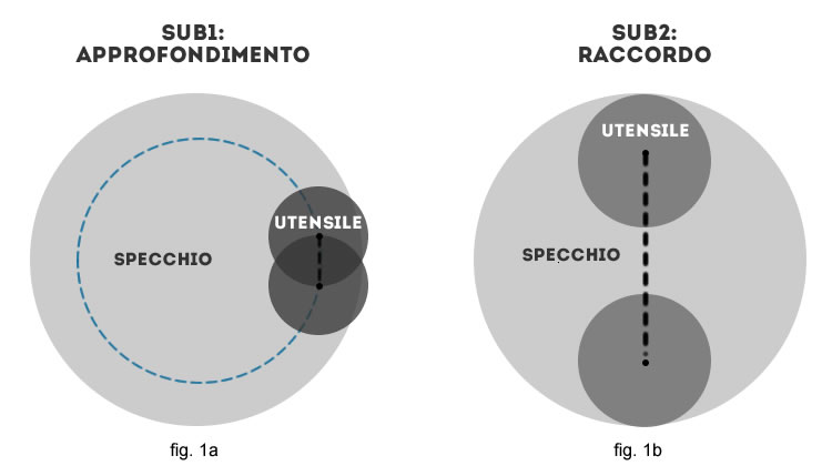
We can say , even if improperly, works :

• The SUB 1 It increases the depth of the outer zones, with a tool to 30% by means of tangential racing.
• the SUB2 “raccorda” deepening newly generated with the complementary deepening of the central areas and medians, using a tool between the 40 and the 50% diameter with central races.
• The SUB3 ( TO BE USED ONLY IN’ LAST PHASE ) It will be the tool to 20% with which we apply the technique described in the preceding article, namely, the exclusive processing of the single zone to increase or decrease the curvature , by means of tangential racing .

We will see later on how and when to apply them in practice, for now let us reflect on planning sessions “combined” with the two tools by introducing also the number of zones with which virtually divide our mirror and the related verification and analysis test.

PLANNING OF WORK

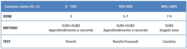
Tabella1

As mentioned, good part of the work will be done with the use of the two techniques combined depth and fitting and only in the very last phase, when the necessary corrections will be of the order of a few hundred nanometers and tests will be carried out with the caustic test, we can use the method previously studied as, at that point, we will necessarily work zones individually ( is increasing that decreasing the curvature ) to reach the end parable.
From the table setting it is clear that our main reference will be the value of the conical constant, that will allow us to compare the analysis of our surface with that of a software simulation, for each value of K between 0 e -1.
The purpose of this method is in fact what never to stray from the conical reference throughout the processing , result obtained by adding to each of the periphery curvature increase, the corresponding depth of the central areas .

BEGINNING AND INTERMEDIATE

After having reached the mirror spherical shape , and having prepared the sub-tools necessary, We begin to deepen the surface:

• With the SUB1 positioned as in fig. 1until ( for a mirror 300 mm the tool edge protrudes 5-6 mm on the edge mirror ) We perform short strokes with light pressure at the center, with constant rotation around the mirror and the rotation of the sub-diameter in the opposite direction each 5-10 past.
• At the end of the session with the SUB1, We change the tool positioning it as shown in fig 1b and execute it with the SUB2 central rides up to the edge mirror ( never go beyond it ) always with light pressure at the center and slow rotation and constant operator around the table and rotation of the on-diameter in the opposite direction each 5-10 past.

TIMES OF SESSIONS

At first the working time for the SUB1 and the SUB2 may be similar. Proceeding with the deepening of the peripheral zone with SUB1, the times of sessions with the SUB2 They will gradually increase and may reach even higher values ​​of 5-6 times.
This simple procedure will, with a little’ of luck, sufficient to bring us close enough to the final parable with a good correction and regularity of the surface, if we have already tested often with the tests and be ready to intervene “targeted adjustments” whenever it presents a deviation from the parable ( conical ) provisional. Let's see how:

SIMULATION AND CHECKS WITH TEST RONCHI *

*We assume that the reader knows how to use the Ronchi test and be able to properly evaluate the results at both theoretical I practice.

Since the checks are always referred to the edge, in the first phase we will just have to assess whether we are working too ( or too little ) with the SUB2 , but beware: we are working on a short-throw , our Ronchi grating You will have a number of linee/mm very low, no more than four , while focal “extreme” below F3 You will need a sun pattern 2 linee/mm or we will find ourselves in a position to show a figure difficult to interpret, almost illegible:

Fig. 2 – Display Differences in the Ronchi test for one F2.5 Mirror – Left: lattice 4 lines / mm Right: lattice 2 linee/mm.

then we perform the Ronchi test and try to identify which of conical constant value is reached by the working. We seek, in accordance with our starting premise , to report the evaluation to the edge always identify ie, for which the value of the conical constant the inclination of the edge bands is similar in test and simulation software.

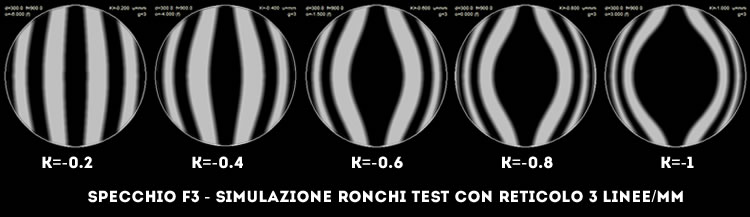
Fig. 3 – Ronchi test for decreasing values ​​of K.

suppose we have assessed it to be very close to the constant K =-0.4 , at this point we evaluate the rest of the figure on the remaining two reference zones:

ANALYSIS AND CONTROL OF PROCESSING

if the rest of the surface has a pattern similar to that of the simulation can consider ourselves lucky ( We guessed the exact relationship between sessions with SUB1 e SUB2 ) and continue deepening until the next evaluation step, otherwise it will occur in the following cases:

1. relative to the periphery, the rest of the surface is shallow: continue for a few sessions only SUB2
2. relative to the periphery, the rest of the surface is too deep: We continue for a few sessions only with the SUB1

These are the most immediate cases that will give us an indication of how we will have to intensify or decrease the machining with the SUB2 as we proceed with the deepening of the periphery with the SUB1.
Our aim is to work, however, maintaining the shape as close as possible to that of reference, although still “fierce” in the values ​​of the conic constant. So going forward, we will begin to carry out the assessments on three areas: peripheral, median and central.
These three areas will be sufficient to achieve the purpose at least until a constant conical K=-0.7 , beyond this value we will have to increase the number of zones and to use the measures for the Foucault test.
In reference to the three areas mentioned, we will begin to carry out the assessments try to identify any defects, assuming as always, that the value of the conical constant reference ( that shows us where we are in the process of building ) It must come from the evaluation of the peripheral zone.
With these assumptions will occur the following defects and interventions described in the table may be adopted 2:

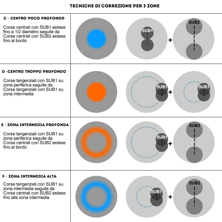
Table 2

should be noted that all the corrective actions described add depth to the figure, therefore they may be used only in the initial and intermediate phase, that is, until our provisional figure will have a reserve of material available to be thorough without exceeding the final design values. For this reason the joints 90% ( or also 95%, if we have been good and lucky ) we will have to abandon the processing part in the method and to intervene directly on the individual zones, but we still generated a very next figure to the final devoid of zonal errors , rugosity, pits and “steps”, all defects easily obtainable working exclusively with small tools on individual areas for prolonged periods.

ADVANCED STAGE, USING EDDY *

*Is’ necessary that the reader knows how to perform the Foucault test with of Couder mask and be able to properly evaluate the results through the software analysis or manual calculation.

Once at 70% of the working or, if you prefer, the conic constant (estimated) of K=-0.7, The Ronchi test can only help in the overall assessment of the surface, to highlight any issues related to roughness, astigmatism, grooves or any other possible local fault though, the machining of the central type and diameter to all performed with the SUB2, It should keep us away from this kind of “surprises”.
Is’ therefore necessary to begin to perform quantitative assessments that give us the measure of the values ​​achieved in the construction of the parable.
To do this we will use the Foucault test with Couder mask with a not high number of zones (5-7), already knowing that this test can not, however, accompany until the end of the machining *, but it will allow us much closer to what will be the end parable.

*the reasons for which the Foucault Test is not able to return a sufficiently correct analysis for parabolic mirrors with F<4 They are highlighted in the article on of Caustic Test

WHY’ 5-7 ZONE

The focal thrust of our mirror will never allow you to view the classic dimming “penumbra” , simultaneous and homogeneous, the opposing areas in the Couder mask indeed, as the focal is short, more able to identify with precision the line of “terminator”, the border area between light and shadow that, in these conditions, It makes it more difficult to assess when it is in the center of curvature of the zone under examination.

What we must consider is this fact when “terminator” crosses the opposing windows simultaneously, namely, enters and exits simultaneously in opposite windows of the same area. In the video evaluation just described is performed on the third zone from the edge, in a mirror 300 F2.6

.
Given that our measures will always be a little’ “approximated” and even more dependent on the operator's sensitivity (both for the objective difficulties of assessment for the inherent limitations of the Foucault test with short focal lengths or very short ) It does not help us increase the number of the areas in question , It might as well keep “low” and use of a minimum of 5 zones for a F4 to a maximum of 7 areas for a F2.

LAST STEP IN-DEPTH

With these assumptions, we are ready to perform the last step in deepening before the final stage of “tweaks”: our goal is to reach or slightly exceed the value of the conic constant we will fix that for the time being K=-0,9 using the Foucault test set to this value, pretending ( limited to this stage ) that our final parable is exactly one corresponding to the value of K=-0.9*

*some authoritative texts suggest to continue using the Foucault test until the final parable ( K=-1) and the achievement of a correction of lambda/4 before switching to the test Caustic. In this article it was decided to restrict the use of Foucault test to the values ​​indicated as the magnitude of the approximation errors and evaluation is dependent on the skill and experience of the operator and could easily lead to much higher error correction request lambda/4, with the risk of being left with a parable, at the time of the final assessment with the most objective and reliable test of the caustic, the value might have already crossed the K parabolic. At that point it would be necessary “come back” and start working sull'abbattimento edge, What definitely doable but would eliminate the very end our starting assumption that has so far provided us with a correct edge to define and to which we have referred all other measures.

We begin therefore to further deepen the periphery according to the usual procedures SUB1 + SUB2, with the variant that from now onwards sessions with SUB1 e SUB2 They will be equal number.

We will continue the sessions even to the outer zones within the tolerance curve (with SUB1 ) without renouncing to a further small central deepening and maintaining the curve with a good coupling between the various zones (with SUB2)

When you have reached the required depth for the suburbs , will move the trajectory of the SUB1 over successive zones by deepening leaving unchanged the central running session with up to SUB2 also lead this industry in tolerance.

The same procedure will then be repeated in sequence up to the innermost zone.

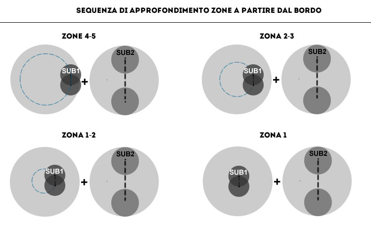
Fig. 4 – Technical depth

Where exactly position the SUB1 after each zonal deepening we will have to decide through the examination of the graph ML .

Is’ important to remember the little “makeup” we defined in Part II of the article ( translation of the ML graph up to bring down the edge of the curve within the tolerance values ) to be able to instantly see what the remaining areas are still “that are high” respect to the edge that we assume correct.

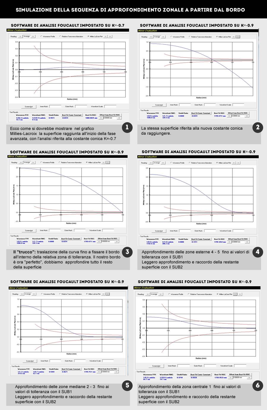
Fig 5 – Simulation of the sequence of deepening in Millies-Lacroix graph with the software Foucault Test Analysis

Is’ good to keep in mind that:

• Given the extent of the SUB1, We will not be able to work a singularly area
• Again follow the general rules on‘increase of the curvature with the sub-diameter .
• The correction techniques described in the case of zonal 3 zones continue to also be applicable in this situation.

At the end of the deepening succession, if we brought all the areas in the vicinity of the tolerance trumpet, we will have a conical slightly sottocorretta than the end parable, and it has maintained its regularity and surface uniformity, ready to be finalized with a few tweaks with the small-diameter sub (SUB3) .

In the fourth and final part will devote ourselves to the achievement of the final parable with particular attention to the practical use of the Test of Caustic.